❌

Reading view

There are new articles available, click to refresh the page.

The Android lockdown seems under-theorized

When you get a cold, the virus hijacks your cells and uses them to make copies of itself, destroying the cells in the process. The virus does not care about you. And yet, if you get a cold, your body doesn’t dissolve into a pile of virus-enriched goo as a result of all your cells disregarding survival to focus on virus manufacturing.

Why? Well, you have an immune system. But also, if that did happen, other people would say, “Oh no, Alice has dissolved into a pile of virus-enriched goo; we should stay away lest we also become goo piles.” Better to just hijack some of your cells, so you can walk around and spread the virus to other people. Thus, the theory of optimal virulence says that a more laid-back cold virus will be more successful in the long run, which is why the cold viruses that thrive today are the non-goo-pile-converting kind.

Anyway. Most people reading this have paid Apple $400-$1600 for a phone on which you can’t do anything without Apple’s permission and monitoring. That was a strange decision, but on Android phones you can run whatever you want. For example, I noticed a couple of months ago that all RSS apps were terrible, so I spent 15 long minutes having AI make me a non-terrible one. I copied the file to my phone, installed it, and entered RSS nirvana, no registration, no app store, no nothing. It seems ludicrous that I wouldn’t be able to do that.

And yet, Google plans to change things. Soon, you won’t be able to run any app on an Android phone unless the person who made it bends the knee by paying a fee, giving Google their government ID, listing all apps they’ve ever made, etc. There will be an “escape hatch” for users to install other apps, but it involves secret menus and scary warnings and a 24-hour waiting period. Google says they’re doing this for security reasons, to prevent people from installing malware that does things like steal financial information.

Three things that any credible analysis of this situation must acknowledge

  1. The security issue is real, and this change will help. Lots of people are in fact getting tricked into installing malware on their phones, and common sense says that this will accelerate with AI. Common sense also says that during that 24-hour waiting period, some of those people might wonder if it’s really normal for OfficialMicrosoftSupportProfessional021 to contact them on WhatsApp to send totally-safe-virus-scanner.apk. It would be convenient for lockdown opponents if the security issue was fake, but it isn’t.

  2. For 95% of people reading this, these restrictions would not be a big deal. You click a few buttons, wait 24 hours once, and then you have the same freedom you have now. That’s still far better than Apple phones where there is no process at all. Oddly, it’s also better than Apple computers, where installing programs from non-verified developers has all sorts of friction that can never be removed. Most people I know use Apple computers anyway and just tolerate the indignity.

  3. If Google cared about freedom or privacy, they could have achieved their security goals without as much harm to freedom or privacy. For example, instead of making themselves the sole arbiter, they could have allowed for multiple certifying entities, and could have allowed users to add others (perhaps after a 24-hour waiting period). Arguably, that would be more secure: That way, grandma could install my RSS app without leaving herself open to random malware. Or, Google could have used private on-device malware scanning, or lots of other things. Google didn’t do that because they don’t care about freedom and privacy and because they like money.1

I think that’s a fair summary. This change addresses a real issue, but it does so in a self-serving way that needlessly destroys freedom. Even so, it only destroys a bit of freedom. This change, by itself, isn’t really a huge deal.

Reading between the lines, I think the real concern is what this might portend. Having made this change, maybe Google will gradually add further restrictions, slowly boiling the frog and moving ever-closer to an Apple-style dictatorship.

But will they? Maybe! Still, this whole situation seems under-theorized. There are good reasons to think that a full lockdown would not be in Google’s interest. And if you care about digital freedom, you could argue that a full lockdown would be a good thing.

Some other analogies

Switching insurance sucks, so some insurers offer a low initial rate and then gradually raise it over time. But they don’t want to raise it too much. Maybe they can charge you $50 more per year than a competitor, because it’s not worth your time to switch to save $50. But if they tried to charge you $5000 more per year, you’d be gone.

Or try this: Say it’s 1750 AD and you’re the King of France. You care nothing about your subjects and only want to extract the maximum possible loot for yourself, no offense Louis XV. How high should you set taxes? High, because you want loot. But not too high, because you don’t want your subjects to revolt and kill you. But still pretty high, because revolting is hard, and your subject know that even if they succeed, they might just end up with another ruler that’s just as rapacious as you.

Or: Say you put a frog in a pot of water and slowly heat it up. What do you think actually happens?

Back to phones

Why are there no Linux phones?

OK, technically there are Linux phones. There are various Linux phone operating systems (PureOS, postmarketOS, Mobian, Manjaro Mobile, Fedora Mobility, openSUSE Mobile) as well as sorta-Linux-sorta-Android operating systems (Ubtuntu touch, Droidian, FuriOS, Sailfish OS) and manufacturers who support them (Purism, Pine, Fairphone, Shift, FuriLabs, {J,V}olla). While I love and support these (♡), the general consensus is that they don’t currently offer an experience that’s remotely comparable to stock Android or iOS, especially for the price.

(Even more technically, Android is itself a kind of Linux, but you know what I mean.)

Obviously, the laws of physics do not forbid Linux phones from being just as good and cheap as an Android phone. They currently aren’t because:

  1. Making cheap phones requires huge economies of scale.
  2. Making a good operating system requires a huge amount of work.
  3. For a phone to be useful it needs good apps, which requires a huge amount of work.

Linux phones don’t have those economies of scale because few people buy them. So, there isn’t enough money to pay people to perfect the operating systems, and most companies don’t bother making apps, and so few people buy those phones.

Meanwhile, there are also various Android-except-de-Googled phone operating systems (LineageOS, GrapheneOS, /e/OS, CalyxOS), and the consensus is that these do come reasonably close to the experience of stock Android or iOS.

Personally, I used Android for a long time while trying to disable as much of Google’s apps and telemetry as I could. A while ago, I got fed up with this and switched to Graphene, one of the most popular Android-except-de-Googled variants. I don’t enjoy tech support bullshit, so I expected some pain, but I was willing to tolerate it for freedom/privacy/whatever. In practice, I found that everything was easy and worked flawlessly and there was no pain at all. Using Graphene made me realize that I had forgotten what it feels like to be “respected” by technology.

So, on a personal level, I recommend that you use Graphene. But this whole situation is full of weird tensions. For one thing, the Graphene project depends on Google for the base of their operating system, and only really survives because of Google’s tolerance. And, at the moment, the only way to use Graphene is to… buy a phone made by Google.

And while I recommend you use Graphene, what I’d prefer you do is switch to a true Linux phone. That would mean that you pay a lot of money for a poor phone experience. But it would help grow the Linux phone ecosystem. If enough people did that, then Linux phones might become become good enough that selfish people like me would switch, further growing the Linux phone ecosystem, et cetera.

That seems unlikely, because digital freedom weirdos face a collective action problem: Linux phones are bad and people are selfish, so we keep buying Android phones and Linux phones stay bad.

There are two ways to solve that collective action problem. Either some entity could invest a ton of money to make Linux phones good, or some entity could do something to make Android worse.

The status quo is good for Google

You may already see the argument I’m making here. Currently Android is just open enough that weirdos like me can run a variant that gives us most of what we want. But doing that is annoying enough that 99.9% of people don’t. This gives Google almost all the benefits of full control, while also sucking up all the oxygen and preventing a real alternative from emerging.

(Apple, incidentally, is laughing. They get to enjoy a full dictatorship while Google does all the hard work.)

Suppose that in six months, Google decides to escalate the lockdown and completely removes the ability to run independent apps. What then?

In the short-run, not much. Tech freedom weirdos would howl, normies wouldn’t notice, and the world would keep turning. But let’s look at some numbers. A rough estimate is that 3-5 million people currently use private de-Googled Android variants like Lineage or Graphene. That’s a crisp 0.1% of the global Android market. Meanwhile, it’s thought that 300-500 million people install Android apps outside the Google store. (That’s excluding China and things like the Samsung and Epic Games Stores.) The biggest reasons are (i) piracy, (ii) modified YouTube/Spotify/WhatsApp clients, (iii) region-locked games, (iv) forbidden gambling or crypto apps, (v) local sharing to save on mobile data, and (vi; least common) open-source app repositories like F-Droid.

In an escalated lockdown, some of this might still be allowed, e.g. local sharing. And many people would simply accept the new restrictions. But I expect that a substantial number would suddenly become interested in de-Googled Android variants that don’t enforce the lockdown. That would be dangerous for Google: If a significant fraction of those 300-500 million people switched, there’s a risk of a vicious/virtuous cycle, where people tell their friends, manufacturers start to cater to those variants, and so on.

If that happened, what would Google do? Might they clamp down on those Android variants, too? Again, maybe! Technically, Android is open-source, but if Google really wanted to kill Lineage or Graphene, there are about 200 different ways they could do that.

So say they did. What would the people currently using those variants do? Again, many would simply submit. That’s good for Google. Others would decide that if they must have an overlord, they’d prefer Apple. That’s not good for Google, but probably not a huge problem given the numbers. But others would decide to look elsewhere, likely to true Linux phones.

Currently, it’s estimated that less than 100 thousand people daily-drive true Linux phones, 30-50 times less than the number of people who use de-Googled Android variants. I’m too lazy and selfish to use a Linux phone now, but Google will take my RSS app from my cold dead hands, so in this scenario, I’d likely switch. If a fraction of people do that—or even get a second Linux phone—it would still represent a huge infusion of money and energy into the Linux phone ecosystem. If this pushed Linux phones from “bad” to “sort of OK”, that could kick off a growth cycle. Eventually, there would be a risk that Europe—eager to decouple from an unreliable US—might embrace them by mandating that government employees use them, or passing a law that popular apps must provide a web-app version that works on Linux phones, or whatever.

Would that actually happen? I don’t know, but neither does Google. My point is that the downside risk of losing their phone duopoly seems vastly larger than the upside, so why risk it? The smart move is to crush alternative app stores and fight malicious apps while making the bare minimum concessions to keep the freedom and privacy people onside. That’s exactly what what Google appears to be doing.

Of course, they might go for a full lockdown anyway. Corporations do dumb things all the time. But I really don’t see how it would be in their self-interest, and I’m not sure it would be a bad thing if they did.

  1. Dynomight: could google achieve the security aims of the android lockdown without so much harm to freedom or privacy

    Google Gemini 4: Yes. Security experts, privacy advocates, and open-source developers widely agree that Google’s primary security objectives—protecting users from malware, financial fraud, spyware, and social engineering—can be achieved through architectural containment, transparent auditing, and informed consent rather than centralized gatekeeping and surveillance. […] The reason Google chooses centralized lockdown over user-controlled security is largely economic and strategic, not technical:

    1. Ecosystem Lock-in: Tying security APIs (like Play Integrity) to Google Play Services makes it nearly impossible for competitors or open-source forks to build a viable alternative Android ecosystem that supports banking and media apps.
    2. Advertising Revenue: Features that dramatically improve both security and privacy—like a native network firewall, revocable internet permissions, or frictionless support for system-wide ad blockers—directly threaten Google’s primary revenue stream.
    3. Liability & Support Reduction: Treating all users as untrusted and removing root/power-user capabilities reduces the surface area of user error, even if it removes the user’s ownership of their own hardware.

    ↩

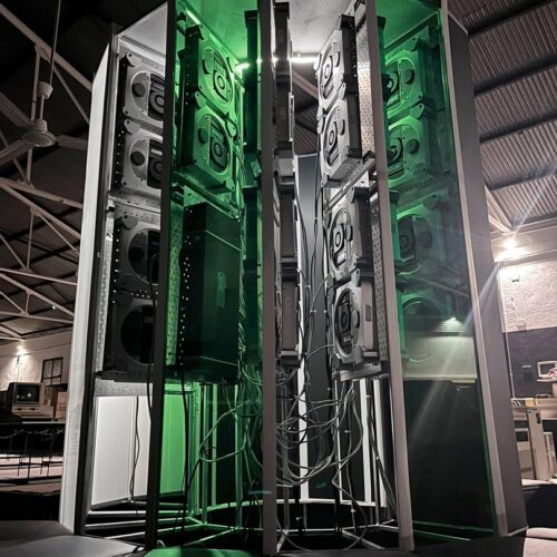
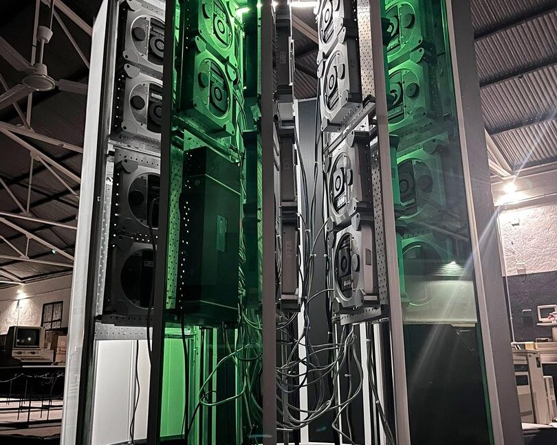
A Cray-1 supercomputer replica from 30 "obsolete" Mac Minis

The Museo de Historia de la Computación in Spain has unveiled a 1:1 scale visual replica of the famous Cray-1 supercomputer from 1976. Instead of sourcing expensive, cutting-edge tech to run the system, the creative team powered the project with 30 2012-era Mac Minis. Developed over 18 months, the project serves as a 50th-anniversary tribute to the Cray-1 and Apple's founding.

Mac Minis from over a decade ago might not seem like the obvious first choice for building a cluster supercomputer, but when networked together, the developers can orchestrate the 64 active processing cores into a combined 1.3 teraflops of performance in their most recent tests. The museum reportedly achieved 1.5 teraflops previously using all 70 available cores, prior to one node going offline. Benchmarks were obtained using a custom matrix-multiplication Python script. Five PCs are quad-core i7s, and the remaining 25 are dual-core i5 models. Except for two units from 2014, the rest of the array dates to 2012.

The replica is a valuable tool for museum-goers to understand the shifts in computer architecture since 1976. The original Cray-1 used vector processing, applying a single instruction to multiple data elements simultaneously, whereas the replica distributes work across independent processors in a parallel cluster. The peak theoretical performance of the original Cray-1 was approximately 160 megaflops. What was originally a purpose-built research machine has been re-created with consumer hardware that's vastly more capable than the machine that inspired it.

Read full article

Comments

DumPy: NumPy except it’s OK if you’re dum

What I want from an array language is:

  1. Don’t make me think.
  2. Run fast on GPUs.
  3. Really, do not make me think.
  4. Do not.

I say NumPy misses on three of these. So I’d like to propose a “fix” that—I claim—eliminates 90% of unnecessary thinking, with no loss of power. It would also fix all the things based on NumPy, for example every machine learning library.

I know that sounds grandiose. Quite possibly you’re thinking that good-old dynomight has finally lost it. So I warn you now: My solution is utterly non-clever. If anything is clever here, it’s my single-minded rejection of cleverness.

To motivate the fix, let me give my story for how NumPy went wrong. It started as a nice little library for array operations and linear algebra. When everything has two or fewer dimensions, it’s great. But at some point, someone showed up with some higher-dimensional arrays. If loops were fast in Python, NumPy would have said, “Hello person with ≥3 dimensions, please call my ≤2 dimensional functions in a loop so I can stay nice and simple, xox, NumPy.”

But since loops are slow, NumPy instead took all the complexity that would usually be addressed with loops and pushed it down into individual functions. I think this was a disaster, because every time you see some function call like np.func(A,B), you have to think:

  1. OK, what shapes do all those arrays have?
  2. And what does np.func do when it sees those shapes?

Different functions have different rules. Sometimes they’re bewildering. This means constantly thinking and constantly moving dimensions around to appease the whims of particular functions. It’s the functions that should be appeasing your whims!

Even simple-looking things like A*B or A[B,C] do quite different things depending on the starting shapes. And those starting shapes are often themselves the output of previous functions, so the complexity spirals.

Worst of all, if you write a new ≤2 dimensional function, then high-dimensional arrays are your problem. You need to decide what rules to obey, and then you need to re-write your function in a much more complex way to—

Voice from the back: Python sucks! If you used a real language, loops would be fast! This problem is stupid!

That was a strong argument, ten years ago. But now everything is GPU, and GPUs hate loops. Today, array packages are cheerful interfaces that look like Python (or whatever) but are actually embedded languages that secretly compile everything into special GPU instructions that run on whole arrays in parallel. With big arrays, you need GPUs. So I think the speed of the host language doesn’t matter so much anymore.

Python’s slowness may have paradoxically turned out to be an advantage, since it forced everything to be designed to work without loops even before GPUs took over.

Still, thinking is bad, and NumPy makes me think, so I don’t like NumPy.

So what’s the fix?

Here’s my extremely non-clever idea: Let’s just admit that loops were better. In high dimensions, no one has yet come up with a notation that beats loops and indices. So, let’s do this:

  1. Bring back the syntax of loops and indices.
  2. But don’t actually execute the loops. Just take the syntax and secretly compile it into vectorized operations.
  3. Also, let’s get rid of all the insanity that’s been added to NumPy because loops were slow.

That’s basically the whole idea. If you take those three bullet-points, you could probably re-derive everything I do below. I told you this wasn’t clever.

What does it look like?

Suppose that X and Y are 2D arrays, and A is a 4D array. And suppose you want to find a 2D array Z such that Zij = (Yj)T (Aij)-1 Xi. If you could write loops, this would be easy:

import numpy as np
Z = np.empty((X.shape[0], Y.shape[0]))
for i in range(X.shape[0]):
    for j in range(Y.shape[0]):
        Z[i,j] = Y[j] @ np.linalg.solve(A[i,j], X[i])

That’s not pretty. It’s not short or fast. But it is easy!

Meanwhile, how do you do this efficiently in NumPy? Like this:

AiX = np.linalg.solve(A.transpose(1,0,2,3),
                      X[None,...,None])[...,0]
Z = np.sum(AiX * Y[:,None], axis=-1).T

If you’re not a NumPy otaku, that may look like outsider art. Rest assured, it looks like that to me too, and I just wrote it. Why is it so confusing? At a high level, it’s because np.linalg.solve and np.sum and multiplication (*) have complicated rules and weren’t designed to work together to solve this particular problem nicely. That would be impossible, because there are an infinite number of problems. So you need to mash the arrays around a lot to make those functions happy.

Without further ado, here’s how you solve this problem with DumPy (ostensibly Dynomight NumPy):

import dumpy as dp
A = dp.Array(A)
X = dp.Array(X)
Y = dp.Array(Y)
Z = dp.Slot()
Z['i','j'] = Y['j',:] @ dp.linalg.solve(A['i','j',:,:], X['i',:])

Yes! If you prefer, you can also use this equivalent syntax:

Z = dp.Slot()
with dp.Range(X.shape[0]) as i:
    with dp.Range(Y.shape[0]) as j:
        Z[i,j] = Y[j,:] @ dp.linalg.solve(A[i,j,:,:], X[i,:])

Those are both fully vectorized. No loops are executed behind the scenes. They’ll run on a GPU if you have one.

But how?

While it looks magical, the way this actually works is fairly simple:

  1. If you index a DumPy array with a string (or a dp.Range object), it creates a special “mapped” array that pretends to have fewer dimensions.

  2. When a DumPy function is called (e.g. dp.linalg.solve or dp.matmul (called with @)), it checks if any of the arguments have mapped dimensions. If so, it automatically vectorizes the computation, matching up mapped dimensions that share labels.

  3. When you assign an array with mapped dimensions to a dp.Slot, it “unmaps” them into the positions you specify.

No evil meta-programming abstract syntax tree macro bytecode interception is needed. When you run this code:

Z = dp.Slot()
Z['i','j'] = Y['j',:] @ dp.linalg.solve(A['i','j',:,:], X['i',:])

This is what happens behind the scenes:

a = A.map_axes([0, 1], ['i', 'j'])
x = X.map_axes([0], ['i'])
y = Y.map_axes([0], ['j'])
z = y @ dp.linalg.solve(a, x)
Z = z.unmap('i','j')
(Click here for a version with a million asserts and comments.)
# first map A
a = A.map_axes([0, 1], ['i', 'j'])
assert A.ndim == 4
assert a.ndim == 2             # pretends to have fewer dims
assert a.data.shape == A.shape          # secret mapped data
assert a.axes == ('i', 'j', None, None) # secret mapped axes
assert a.shape == (a.data.shape[2], a.data.shape[3])
                # shape determined by non-mapped (None) axes

# now map X
x = X.map_axes([0], ['i'])
assert X.ndim == 2
assert x.ndim == 1
assert x.data.shape == X.shape
assert x.axes == ('i', None)
assert x.shape == (x.data.shape[1], )

# now map Y
y = Y.map_axes([0], ['j'])
assert Y.ndim == 2
assert y.ndim == 1
assert y.shape == (Y.shape[1],)
assert y.axes == ('j', None)
assert y.data.shape == Y.shape
assert y.shape == (y.data.shape[1],)

# Actually do the computation. It happens that the 'j'
# dimension is stored first because its found first (in y).
# But you never need to think about that!
z = y @ dp.linalg.solve(a, x)
assert z.ndim == 0
assert z.shape == ()
assert z.axes == ('j','i')
assert z.data.shape == (Y.shape[0], X.shape[0])

# unmap the mapped axes
Z = z.unmap('i','j')
assert Z.ndim == 2
assert Z.shape == (X.shape[0], Y.shape[0])

Wait, but how?

It might seem like I’ve skipped the hard part. How does dp.linalg.solve know how to vectorize over any combination of input dimensions? Don’t I need to do that for every single function that DumPy includes? Isn’t that hard?

It is hard, but jax.vmap did it already. This takes a function defined using (JAX’s version of) NumPy and vectorizes it over any set of input dimensions. DumPy relies on this to do all the actual vectorization. (If you prefer your vmap janky and broken, I heartily recommend PyTorch’s torch.vmap.)

But hold on. If vmap already exists, then why do we need DumPy? Here’s why:

import jax
from jax import numpy as jnp
Z = jax.vmap(
        jax.vmap(
            lambda x, y, a: y @ jnp.linalg.solve(a, x),
            in_axes=[None, 0, 0]
        ),
        in_axes=[0, None, 0]
    )(X, Y, A)

That’s how you solve the same problem with vmap. (And basically what DumPy does behind the scenes.)

I think vmap is one of the best parts of the NumPy ecosystem. The above code seems genuinely better than the base NumPy version. But it still involves a lot of thinking! Why put in_axes=[None, 0, 0] in the inner vmap and in_axes=[0, None, 0] in the outer one? Why are all the axes 0 even though you need to vectorize over the second dimension of A? There are answers, but they require thinking. Loops and indices are better.

A tiny bit of cleverness

OK, I did do one thing that’s a little clever. Say you want to create a Hilbert matrix with Hij = 1/(1+i+j). In base NumPy you’d have to do this:

X = 1 / (1 + np.arange(5)[:,None] + np.arange(5)[None,:]) # hurr?

In DumPy, you can just write:

X = dp.Slot()
with dp.Range(5) as i:
    with dp.Range(5) as j:
        X[i,j] = 1 / (i + j + 1)

Yes! That works! It works because a dp.Range acts both like a string and like an array mapped along that string. So the above code is roughly equivalent to:

I = dp.Array([0,1,2,3,4])
J = dp.Array([0,1,2,3,4])
X = dp.Slot()
X['i','j'] = 1 / (1 + I['i'] + J['j'])
See? Still no magic.

In reality, the dp.Range choose random strings. (The class maintains a stack of active ranges to prevent collisions.) So in more detail, the above code becomes something like this:

I = dp.Array([0,1,2,3,4])
J = dp.Array([0,1,2,3,4])
i = I.map_axes([0],'range_EZaW')
j = J.map_axes([0],'range_ailw')
x = 1 / (1 + i + j) # vectorized
X = x.unmap('range_EZaW','range_ailw')

OK but is it actually better?

To test if DumPy is actually better in practice, I took six problems of increasing complexity and implemented each of them using loops, NumPy, JAX (with vmap), and DumPy.

Hilbert matrices

Note that in these examples, I always assume the input arrays are in the class of the system being used. If you try running them, you’ll need to add some conversions with np.array / jnp.array / dp.Array.

# loops
H = np.empty((N, N))
for i in range(N):
    for j in range(N):
        H[i, j] = 1 / (i + j + 1)

# NumPy
i = np.arange(N)
j = np.arange(N)
H = 1 / (i[:, None] + j[None, :] + 1)

# JAX
indices = jnp.arange(N)
H = jax.vmap(
        jax.vmap(
            lambda i, j: 1 / (i + j + 1),
            [0, None]),
        [None, 0]
    )(indices, indices)

# DumPy
H = dp.Slot()
with dp.Range(N) as i:
    with dp.Range(N) as j:
        H[i, j] = 1 / (i + j + 1) # Yes! This works!
Batched covariance
# Loops
C = np.zeros((X.shape[0],X.shape[1],X.shape[1]))
for n in range(X.shape[0]):
    C[n] = np.cov(X[n])

# NumPy
mu = np.mean(X, axis=2)[:, :, None]    # hurr?
C = np.sum((X - mu)[:, None, :, :] *
           (X - mu)[:, :, None, :],
           axis=3) / (X.shape[2] - 1)  # hurrr??

# JAX
C = jax.vmap(jnp.cov)(X)

# DumPy
C = dp.Slot()
with dp.Range(X.shape[0]) as n:
    C[n, :, :] = dp.cov(X[n, :, :])

# DumPy (alternate)
C = dp.Slot()
C['n',:,:] = dp.cov(X['n',:,:])
Moving average

(Pretending numpy.lib.stride_tricks doesn’t exist.)

# Loops
B = np.empty(N - window + 1)
for i in range(N - window + 1):
    B[i] = np.mean(A[i:i + window])

# NumPy
i = np.arange(N - window + 1)[:, None]
j = np.arange(window)[None, :] 
B = np.mean(A[i+j], axis=-1)

# JAX
idx = jnp.arange(window)
B = jax.vmap(
        lambda i: jnp.mean(A[i+idx]),
    )(jnp.arange(N - window + 1))

# DumPy
windowed = dp.Slot()
B = dp.Slot()
with dp.Range(N - window + 1) as i:
    with dp.Range(window) as j:
        windowed[i, j] = A[i + j]
    B[i] = dp.mean(windowed[i, :])
    # Note: B[i] = dp.mean(A[i:i+window])
    # would not work because dp.Range can't be used in slice
Indexing

The goal is to create E with

  E[i1, i2, :, i3] = A[B[i1], C[i1, i2], ::2, D[i2, i3]].

# Setup
K = 4
L = 5
M = 6
N = 7

A = np.random.randn(K, L, M, N)
B = np.random.randint(0, K, size=(9,))
C = np.random.randint(0, L, size=(9, 10))
D = np.random.randint(0, N, size=(10, 11))

# Loops
E = np.empty((9, 10, M // 2, 11))
for i1 in range(9):
    for i2 in range(10):
        for i3 in range(11):
            E[i1,i2,:,i3] = A[B[i1],C[i1, i2],::2,D[i2, i3]]

# NumPy
E = A[B[:, None, None],
      C[:, :, None],
      ::2,
      D[None, :, :]
    ].transpose((0, 1, 3, 2))

# JAX
E = jax.vmap(
        jax.vmap(
            jax.vmap(
                lambda b, c, d: A[b, c, ::2, d],
                in_axes=[None,None,0]),
            in_axes=[None,0,0]),
        in_axes=[0,0,None]
    )(B,C,D).transpose(0,1,3,2)

# DumPy
E = dp.Slot()
with dp.Range(9) as i1:
    with dp.Range(10) as i2:
        with dp.Range(11) as i3:
            E[i1,i2,:,i3] = A[B[i1],C[i1, i2],::2,D[i2, i3]]

# DumPy (alternative)
E = dp.Slot()
E['i1','i2',:,'i3'] = A[B['i1'], C['i1','i2'], ::2, D['i2','i3']]

Gaussian Densities

The goal of this problem is, given a list of vectors and a list of Gaussians parameters, and arrays mapping each vector to a list of parameters, evaluate each corresponding vector/parameter combination. Formally, given 2D X, B, C, and means and 3D covs, the goal is to create A with

  Aij = log N( Xi | meansBij, covsCij) .

# Setup
ndims = 3
ndata = 10
neval = 5
ndist = 7

X = np.random.randn(ndata, ndims)
B = np.random.randint(0, ndist, size=(ndata, neval))
C = np.random.randint(0, ndist, size=(ndata, neval))
means = np.random.randn(ndist, ndims)
scales = np.array(np.random.randn(ndist, ndims, ndims))
covs = np.array([scale @ scale.T for scale in scales])
# Loops
def log_prob(x, mean, cov):
    diff = x - mean
    y = np.linalg.solve(cov, diff)
    quad = diff @ y
    logdet = np.linalg.slogdet(2 * np.pi * cov)[1]
    return -0.5 * (quad + logdet)

A = np.empty((ndata, neval))
for i in range(ndata):
    for j in range(neval):
        A[i, j] = log_prob(X[i, :],
                           means[B[i, j], :],
                           covs[C[i, j], :, :])

# NumPy
diff = X[:, None, :] - means[B]
y = np.linalg.solve(covs[C], diff[..., None])
quad = np.sum(diff * y[..., 0], axis=-1)
logdet = np.linalg.slogdet(2 * np.pi * covs[C])[1]
A = -0.5 * (quad + logdet)

# JAX
A = jax.vmap(
        jax.vmap(
            log_prob_gauss,
            in_axes=[None, 0, 0]
        ),
    )(X, means[B], covs[C])

# DumPy
def log_prob(x, mean, cov):
    diff = x - mean
    quad = diff @ dp.linalg.solve(cov, diff)
    logdet = dp.linalg.slogdet(2 * jnp.pi * cov)[1]

A = dp.Slot()
with dp.Range(ndata) as i:
    with dp.Range(neval) as j:
        A[i, j] = log_prob(X[i,:],
                           means[B[i,j],:],
                           covs[C[i,j],:,:])

# DumPy (alternate)
A = dp.Slot()
with dp.Range(ndata) as i:
    with dp.Range(neval) as j:
        mean = means[B[i,j],:]
        cov = covs[C[i,j],:,:]
        diff = X[i,:] - mean
        quad = diff @ dp.linalg.solve(cov, diff)
        logdet = dp.linalg.slogdet(2 * jnp.pi * cov)[1]
        A[i,j] = -0.5 * (quad + logdet)
Multi-head self-attention

See also the discussion in the previous post.

# Setup
input_dim = 4
seq_len = 4
d_k = 5
d_v = input_dim
n_head = 2
X = np.random.randn(seq_len, input_dim)
W_q = np.random.randn(n_head, input_dim, d_k)
W_k = np.random.randn(n_head, input_dim, d_k)
W_v = np.random.randn(n_head, input_dim, d_v)
W_o = np.random.randn(n_head, d_v, input_dim // n_head)

# Loops
def softmax_numpy(x, axis=-1):
    e_x = np.exp(x - np.max(x, axis=axis, keepdims=True))
    return e_x / np.sum(e_x, axis=axis, keepdims=True)

def attention(X, W_q, W_k, W_v):
    Q = X @ W_q
    K = X @ W_k
    V = X @ W_v
    scores = Q @ K.T / np.sqrt(d_k)
    attention_weights = softmax_numpy(scores, axis=-1)
    output = attention_weights @ V
    return output

def multi_head_attention_loops(X, W_q, W_k, W_v, W_o):
    projected = []
    for n in range(n_head):
        my_output = attention(X,
                                W_q[n, :, :],
                                W_k[n, :, :],
                                W_v[n, :, :])
        my_proj = my_output @ W_o[n, :, :]
        projected.append(my_proj)
    projected = np.array(projected)

    final = []
    for i in range(seq_len):
        my_final = np.ravel(projected[:, i, :])
        final.append(my_final)
    return np.array(final)

# NumPy
def softmax_numpy(x, axis=-1): # repeat
    e_x = np.exp(x - np.max(x, axis=axis, keepdims=True))
    return e_x / np.sum(e_x, axis=axis, keepdims=True)

def multi_head_attention_numpy(X, W_q, W_k, W_v, W_o):
    Q = np.einsum('si,hij->hsj', X, W_q)
    K = np.einsum('si,hik->hsk', X, W_k)
    V = np.einsum('si,hiv->hsv', X, W_v)
    scores = Q @ K.transpose(0, 2, 1) / np.sqrt(d_k)
    weights = softmax_numpy(scores, axis=-1)
    output = weights @ V
    projected = np.einsum('hsv,hvd->hsd', output, W_o)
    return projected.transpose(1, 0, 2).reshape(
        seq_len, input_dim)

# JAX
def softmax_jax(x, axis=-1):
    e_x = jnp.exp(x - jnp.max(x, axis=axis, keepdims=True))
    return e_x / jnp.sum(e_x, axis=axis, keepdims=True)

def attention_jax(X, W_q, W_k, W_v):
    d_k = W_k.shape[-1]
    Q = X @ W_q
    K = X @ W_k
    V = X @ W_v
    scores = Q @ K.T / jnp.sqrt(d_k)
    attention_weights = softmax_jax(scores, axis=-1)
    output = attention_weights @ V
    return output

def multi_head_attention_jax(X, W_q, W_k, W_v, W_o):
    def myfun(X, w_q, w_k, w_v, w_o):
        return attention_jax(X, w_q, w_k, w_v) @ w_o

    projected = jax.vmap(myfun,
                            in_axes=[None, 0, 0, 0, 0]
                )(X, W_q, W_k, W_v, W_o)

    return jax.vmap(jnp.ravel, in_axes=1)(projected)

# DumPy
def softmax_dumpy(x):
    assert x.ndim == 1 # no need to think about dimensions!
    e_x = dp.exp(x - dp.max(x))
    return e_x / dp.sum(e_x)

@dp.wrap # needed to make functions with Slots auto-vectorizing
def attention_dumpy(X, W_q, W_k, W_v):
    Q = X @ W_q
    K = X @ W_k
    V = X @ W_v
    scores = Q @ K.T / np.sqrt(d_k)
    attention_weights = dp.Slot()
    with dp.Range(seq_len) as i:
        attention_weights[i, :] = softmax_dumpy(scores[i, :])
    output = attention_weights @ V
    return output

def multi_head_attention_dumpy(X, W_q, W_k, W_v, W_o):
    output = dp.Slot()
    projected = dp.Slot()
    final = dp.Slot()
    with dp.Range(n_head) as n:
        output[n, :, :] = attention_dumpy(X,
                                          W_q[n, :, :],
                                          W_k[n, :, :],
                                          W_v[n, :, :])
        projected[n, :, :] = output[n, :, :] @ W_o[n, :, :]
    with dp.Range(seq_len) as i:
        final[i, :] = dp.ravel(projected[:, i, :])
    return final

# DumPy (alternate)
def multi_head_attention(X, W_q, W_k, W_v, W_o):
    attn_weights = dp.Slot()
    projected = dp.Slot()
    final = dp.Slot()
    with dp.Range(n_head) as n:
        Q = X @ W_q[n, :, :]
        K = X @ W_k[n, :, :]
        V = X @ W_v[n, :, :]
        scores = Q @ K.T / np.sqrt(d_k)
        with dp.Range(seq_len) as i:
            attn_weights[n, i, :] = softmax_dumpy(scores[i, :])
        projected[n, :, :] = attn_weights[n, :, :] @ V @ W_o[n, :, :]
    with dp.Range(seq_len) as i:
        final[i, :] = dp.ravel(projected[:, i, :])
    return final

I gave each implementation a subjective “goodness” score on a 1-10 scale. I always gave the best implementation for each problem 10 points, and then took off points from the others based on how much thinking they required.

Problem Loops Numpy JAX (vmap) DumPy
Hilbert matrices 10 7 7 10
Covariance 9 4 10 9
Moving Ave. 10 6 6 8
Indexing 10 5 4 10
Gaussians 10 3 6 10
Attention 10 1 8 10
Mean 9.8 4.3 6.8 9.5

According to this dubious methodology and these made-up numbers, DumPy is 96.93877% as good as loops! Knowledge is power! But seriously, while subjective, I don’t think my scores should be too controversial. The most debatable one is probably JAX’s attention score.

What to remove?

The only thing DumPy adds to NumPy is some nice notation for indices. That’s it.

What I think makes DumPy good is it also removes a lot of stuff. Roughly speaking, I’ve tried to remove anything that is confusing and exists because NumPy doesn’t have loops. I’m not sure that I’ve drawn the line in exactly the right place, but I do feel confident that I’m on the right track with removing stuff.

1. Goodbye broadcasting

In NumPy, A*B works if A and B are both scalar. Or if A is 5×1×6 and B is 5×1×6×1. But not if A is 1×5×6 and B is 1×5×6×1. Huh?

In truth, the broadcasting rules aren’t that complicated for scalar operations like multiplication. But still, I don’t like it, because every time you see A*B, you have to worry about what shapes those have and what the computation might be doing.

So, I removed it. In DumPy you can only do A*B if one of A or B is scalar or A and B have exactly the same shape. That’s it, anything else raises an error. Instead, use indices, so it’s clear what you’re doing. Instead of this:

C = A[...,None] * B[None]

write this:

C['i','j','k'] = A['i','j'] * B['j','k']

2. Goodbye fancy indexing

Indexing in NumPy is absurdly complicated. When you write A[B,C,D] that could do many different things depending on what all the shapes are. I considered going cold-turkey and only allowing scalar indices in DumPy. That wouldn’t have been so bad, since you can still do advanced stuff using loops. But it’s quite annoying to not be able to write A[B] when A and B are just simple 1D arrays.

So I’ve tentatively decided to be more pragmatic. In DumPy, you can index with integers, or slices, or (possibly mapped) Arrays. But only one Array index can be non-scalar. I settled on this because it’s the most general syntax that doesn’t require thinking.

Let me show you what I mean. If you see this:

A[1, 1:6, C, 2:10] # legal in both numpy and dumpy

It’s “obvious” what the output shape will be. (First the shape of 1:6, then the shape of C, then the shape of 2:10). Simple enough. But as soon as you have two multidimensional array inputs like this:

A[B, 1:6, C, 2:10] # legal in numpy, verboten in dumpy

Suddenly all hell breaks loose. You need to think about broadcasting between B and C, orthogonal vs. pointwise indices, slices behaving differently than arrays, and quirks for where the output dimensions go. So DumPy forbids this. Instead, you need to write one of these:

D['i',:,:]     = A[B['i'],     1:6, C['i'],     2:10] # (1)
D[:,:,'i']     = A[B['i'],     1:6, C['i'],     2:10] # (2)
D['i','j',:,:] = A[B['i'],     1:6, C['j'],     2:10] # (3)
D['i','j',:,:] = A[B['i','j'], 1:6, C['i'],     2:10] # (4)
D['i','j',:,:] = A[B['i','j'], 1:6, C['i','j'], 2:10] # (5)

They all do exactly what they look like they do.

Oh, and one more thing! In DumPy, you must index all dimensions. In NumPy, if A has three dimensions, then A[2] is equivalent to A[2,:,:]. This is sometimes nice, but it means that every time you see A[2], you have to worry about how many dimensions A has. In DumPy, every time you index an array or assign to a dp.Slot, it checks that all indices have been included. So when you see option (4) above, you know that:

  • A has 4 dimensions
  • B has 2 dimensions
  • C has 1 dimension
  • D has 4 dimensions

Always, always, always. No cases, no thinking.

3. Goodbye complicated functions

Again, many NumPy functions have complex conventions for vectorization. np.linalg.solve sort of says, “If the inputs have ≤2 dimensions, do the obvious thing. Otherwise, do some extremely confusing broadcasting stuff.” DumPy removes the confusing broadcasting stuff. When you see dp.linalg.solve(A,B), you know that A and B have no more than two dimensions, so nothing tricky is happening.

Similarly, in NumPy, A @ B is equivalent to np.matmul(A,B). When both inputs have ≤2 or fewer dimensions, this does the “obvious thing”. (Either an inner-product or some kind of matrix/vector multiplication.) Otherwise, it broadcasts or vectorizes or something? I can never remember. In DumPy you don’t have that problem, because it restricts A @ B to arrays with one or two dimensions only.

If you need more dimensions, no problem: Use indices.

Why remove?

It might seem annoying to remove features, but I’m telling you: Just try it. If you program this way, a wonderful feeling of calmness comes over you, as class after class of possible errors disappear.

Put another way, why remove all the fancy stuff, instead of leaving it optional? Because optional implies thinking! I want to program in a simple way. I don’t want to worry that I’m accidentally triggering some confusing broadcasting insanity, because that would be a mistake. I want the computer to help me catch mistakes, not silently do something weird that I didn’t intend.

In principle, it would be OK if there was a evil_solve method that preserves all the confusing batching stuff. If you really want that, you can make it yourself:

evil_solve = dp.MappedFunction(jnp.linalg.solve) # not recommended

You can use that same wrapper to convert any JAX NumPy function to work with DumPy.

Discussion

Think about math: In two or fewer dimensions, coordinate-free linear algebra notation is wonderful. But for higher dimensional tensors, there are just too many cases, so most physicists just use coordinates.

So this solution seems pretty obvious to me. Honestly, I’m a little confused why it isn’t already standard. Am I missing something?

What about APL?

When I complain about NumPy, many people often suggest looking into APL-type languages, like A, J, K, or Q. (All single-letter languages are APL-like, except C, D, F, R, T, X, and many others. Convenient, right?) The obvious disadvantages of these are that:

  1. They’re unfamiliar.
  2. The code looks like gibberish.
  3. They don’t usually provide autodiff or GPU execution.

None of those bother me. If the languages are better, we should learn to use them and make them do autodiff on GPUs. But I’m not convinced they are better. When you actually learn these languages, what you figure out is that the symbol gibberish basically amounts to doing the same kind of dimension mashing that we saw earlier in NumPy:

AiX = np.linalg.solve(A.transpose(1,0,2,3),
                      X[None,...,None])[...,0]
Z = np.sum(AiX * Y[:,None], axis=-1).T

The reason is that, just like NumPy and vmap, these languages choose align dimensions by position, rather than by name. If I have to mash dimensions, I want to use the best tool. But I’d prefer not to mash dimensions at all.

What about named dimensions?

People also often suggest “NumPy with named dimensions” as in xarray. (PyTorch also has a half-hearted implementation.) Of course, DumPy also uses named dimensions, but there’s a critical difference. In xarray, they’re part of the arrays themselves, while in DumPy, they live outside the arrays.

In some cases, permanent named dimensions are very nice. But for linear algebra, they’re confusing. For example, suppose A is 2-D with named dimensions "cat" and "dog". Now, what dimensions should ATA have? ("dog" twice?) Or say you take a singular value decomposition like U, S, Vh = svd(A). What name should the inner dimensions have? Does the user have to specify it?

I haven’t seen a nice solution. xarray doesn’t focus on linear algebra, so it’s not much of an issue there. A theoretical “DumPy with permanent names” might be very nice, but I’m not sure how it should work. This is worth thinking about more.

What about Julia or [other language]

I like Julia! Loops are fast in Julia! But again, I don’t think fast loops matter that much, because I want to move all the loops to the GPU. So even if I was using Julia, I think I’d want to use a DumPy-type solution.

I think Julia might well be a better host language than Python, but it wouldn’t be because of fast loops, but because it offers much more powerful meta-programming capabilities. I built DumPy on top of JAX just because JAX is very mature and good at calling the GPU, but I’d love to see the same idea used in Julia (“Dulia”?) or other languages.

Prototype

OK, I promised a link to my prototype, so here it is: dumpy.py

It’s just a single file with around 700 lines. I’m leaving it as a single file because I want to stress that this is just something I hacked together in the service of this rant. I wanted to show that I’m not totally out of my mind, and that doing all this is actually pretty easy.

I stress that I don’t really intend to update or improve this. (Unless someone gives me a lot of money?) So please do not attempt to use it for “real work”, and do not make fun of my code.

PS. DumPy works out of the box with both jax.jit and jax.grad. For gradients, you need to either cast the output to a JAX scalar or use the dp.grad wrapper.

PPS. If you like this, you may also like einx or torchdim.


Update: Due to many requests, I have turned this into a “real” package, available on PyPi as dumpy-numpy. You can install it by typing:

pip install dumpy-numpy

Or, if you use uv (you should) you can play around with DumPy by just typing this one-liner in your terminal:

uv run --with dumpy-numpy --with ipython ipython

For example:

UV quickstart

I don’t like NumPy

They say you can’t truly hate someone unless you loved them first. I don’t know if that’s true as a general principle, but it certainly describes my relationship with NumPy.

NumPy, by the way, is some software that does computations on arrays in Python. It’s insanely popular and has had a huge influence on all the popular machine learning libraries like PyTorch. These libraries share most of the same issues I discuss below, but I’ll stick to NumPy for concreteness.

NumPy makes easy things easy. Say A is a 5×5 matrix, x is a length-5 vector, and you want to find the vector y such that Ay=x. In NumPy, that would be:

y = np.linalg.solve(A, x)

So elegant! So clear!

But say the situation is even a little more complicated. Say A is a stack of 100 5×5 matrices, given as a 100×5×5 array. And say x is a stack of 100 length-5 vectors, given as a 100×5 array. And say you want to solve Aᵢyᵢ=xᵢ for 1≤i≤100.

If you could use loops, this would be easy:

y = np.empty_like(x)
for i in range(100):
    y[i,:] = np.linalg.solve(A[i,:,:], x[i,:])

But you can’t use loops. To some degree, this is a limitation of loops being slow in Python. But nowadays, everything is GPU and if you’ve got big arrays, you probably don’t want to use loops in any language. To get all those transistors firing, you need to call special GPU functions that will sort of split up the arrays into lots of little pieces and process them in parallel.

The good news is that NumPy knows about those special routines (at least if you use JAX or CuPy), and if you call np.linalg.solve correctly, it will use them.

The bad news is that no one knows how do that.

Don’t believe me? OK, which of these is right?

y = linalg.solve(A,x)
y = linalg.solve(A,x,axis=0)
y = linalg.solve(A,x,axes=[[1,2],1])
y = linalg.solve(A.T, x.T)
y = linalg.solve(A.T, x).T
y = linalg.solve(A, x[None,:,:])
y = linalg.solve(A,x[:,:,None])
y = linalg.solve(A,x[:,:,None])[:,:,0]
y = linalg.solve(A[:,:,:,None],x[:,None,None,:])
y = linalg.solve(A.transpose([1,2,0]),x[:,:,None]).T

No one knows. And let me show you something else. Here’s the documentation:

np.linalg.solve

Read that. Meditate on it. Now, notice: You still don’t know how to solve Aᵢyᵢ=xᵢ for all i at once. Is it even possible? Did I lie when I said it was?

As far as I can tell, what people actually do is try random variations until one seems to work.

Why NumPy bad

NumPy is all about applying operations to arrays. When the arrays have 2 or fewer dimensions, everything is fine. But if you’re doing something even mildly complicated, you inevitably find yourself with some operation you want to apply to some dimensions of array A, some other dimensions of array B, and some other dimensions of array C. And NumPy has no theory for how to express that.

Let me show you what I mean. Suppose:

  • A is a K×L×M array
  • B is a L×N array
  • C is a K×M array

And say that for each k and n, you’d like to compute the mean over the L and M dimensions. That is, you want

   Dkn = 1/(LM) × ∑lm Aklm Bln Ckm.

To do that, you’ve got two options. The first is to use grotesque dimension alignment tricks:

D = np.mean(
        np.mean(
            A[:,:,:,None] *
            B[None,:,None,:] *
            C[:,None,:,None],
        axis=1),
    axis=1)

The hell, you ask? Why is None everywhere? Well, when indexing an array in NumPy, you can write None to insert a new dimension. A is K×L×M, but A[:,:,:,None] is K×L×M×1. Similarly, B[None,:,None,:] is 1×L×1×N and C[:,None,:,None] is K×1×M×1. When you multiply these together, NumPy “broadcasts” all the size-1 dimensions to give a K×L×M×N array. Then, the np.mean calls average over the L and M dimensions.

I think this is bad. I’ve been using NumPy for years and I still find it impossible to write code like that without always making mistakes.

It’s also borderline-impossible to read. To prove this, I just flipped a coin and introduced a bug above if and only if the coin was tails. Is there a bug? Are you sure? No one knows.

Your second option is to desperately try to be clever. Life is short and precious, but if you spend a lot of yours reading the NumPy documentation, you might eventually realize that there’s a function called np.tensordot, and that it’s possible to make it do much of the work:

D = (1/L) * np.mean(
                np.tensordot(A, B, axes=[1,0]) *
                C[:,:,None],
            axis=1)

That’s correct. (I promise.) But why does it work? What exactly is np.tensordot doing? If you saw that code in some other context, would you have the slightest idea what was happening?

Here’s how I’d do it, if only I could use loops:

D = np.zeros((K,N))  
for k in range(K):  
    for n in range(N):  
        a = A[k,:,:]  
        b = B[:,n]  
        c = C[k,:]  
        assert a.shape == (L,M)  
        assert b.shape == (L,)  
        assert c.shape == (M,)  
        D[k,n] = np.mean(a * b[:,None] * c[None,:])

People who’ve written too much NumPy may find that clunky. I suspect that’s a wee bit of Stockholm Syndrome. But surely we can agree that it’s clear.

In practice, things are often even worse. Say that A had shape M×K×L rather than K×L×M. With loops, no big deal. But NumPy requires you to write monstrosities like A.transpose([1,2,0]). Or should that be A.transpose([2,0,1])? What shapes do those produce? No one knows.

Loops were better.

OK I lied

There is a third option:

D = 1/(L*M) * np.einsum('klm,ln,km->kn', A, B, C)

If you’ve never seen Einstein summation before, that might look terrifying. But remember, our goal is to find

   Dkn = 1/(LM) × ∑lm Aklm Bln Ckm.

The string in the above code basically gives labels to the indices in each of the three inputs (klm,ln,km) and the target indices for the output (->kn). Then, np.einsum multiplies together the corresponding elements of the inputs and sums over all indices that aren’t in the output.

Personally, I think np.einsum is one of the rare parts of NumPy that’s actually good. The strings are a bit tedious, but they’re worth it, because the overall function is easy(ish) to understand, is completely explicit, and is quite general and powerful.

Except, how does np.einsum achieve all this? It uses indices. Or, more precisely, it introduces a tiny domain-specific language based on indices. It doesn’t suffer from NumPy’s design flaws because it refuses to play by NumPy’s normal rules.

But np.einsum only does a few things. (Einops does a few more.) What if you want to apply some other function over various dimensions of some arrays? There is no np.linalg.einsolve. And if you create your own function, there’s certainly no “Einstein” version of it.

I think np.einsum’s goodness shows that NumPy went somewhere.

Intermission

Here’s a painting which feels analogous to our subject.

Where did NumPy go wrong?

Here’s what I want from an array language. I ain’t particular about syntax, but it would be nice if:

  1. When you want to do something, it’s “obvious” how to do it.
  2. When you read some code, it’s “obvious” what it does.

Wouldn’t that be nice? I think NumPy doesn’t achieve these because of its original sin: It took away indices and replaced them with broadcasting. And broadcasting cannot fill indices’ shoes.

I don’t love NumPy broadcasting

NumPy’s core trick is broadcasting. Take this code:

A = np.array([[1,2],[3,4],[5,6]])
B = np.array([10,20])
C = A * B
print(C)

This outputs:

[[ 10  40]
 [ 30  80]
 [ 50 120]]

Here, A is a 3×2 array, and B is a length-2 array. When you multiply them together, B is “broadcast” to the shape of A, meaning the first column of A is multiplied with B[0]=10 and the second is multiplied with B[1]=20.

In simple cases, this seems good. But I don’t love it. One reason is that, as we saw above, you often have to do gross things to the dimensions to get them to line up.

Another reason is that it isn’t explicit or legible. Sometimes A*B multiplies element-by-element, and sometimes it does more complicated things. So every time you see A*B, you have to figure out which case in the broadcasting conventions is getting triggered.

But the real problem with broadcasting is how it infects everything else. I’ll explain below.

I don’t like NumPy indexing

Here’s a riddle. Take this code:

A = np.ones((10,20,30,40))
i = np.array([1,2,3])
j = np.array([[0],[1]])
B = A[:,i,j,:]

What shape does B have?

It turns out the answer is 10×2×3×40. That’s because the i and j indices get broadcast to a shape of 2×3 and then something something mumble mumble mumble. Try to convince yourself it makes sense.

Done? OK, now try these:

C = A[:,:,i,j]
D = A[:,i,:,j]
E = A[:,1:4,j,:]

What shapes do these have?

  • C is 10×20×2×3. This seems logical, given what happened with B above.

  • What about D? It is 2×3×10×30. Now, for some reason, the 2 and 3 go at the beginning?

  • And what about E? Well, “slices” in Python exclude the endpoint, so 1:4 is equivalent to [1,2,3] which is equivalent to i, and so E is the same as B. Hahaha, just kidding! E is 10×3×2×1×40.

Yes, that is what happens. Try it if you don’t believe me! I understand why NumPy does this, because I’ve absorbed this 5000 word document that explains how NumPy indexing works. But I want that time back.

For fun, I tried asking a bunch of AI models to figure out what shapes those arrays have. Here were the results:

I used this query:

Take this python code

A = np.ones((10,20,30,40))
i = np.array([1,2,3])
j = np.array([[0],[1]])
B = A[:,i,j,:]
C = A[:,:,i,j]
D = A[:,i,:,j]
E = A[:,1:4,j,:]

what shapes do B, C, D, and E have?

Claude 3.7 used “extended thinking”. Here are all the incorrect outputs:

AI B C D E
GPT 4.1     10×2×3×30  
Grok 3     10×3×30×2 10×3×2×40
Claude 3 Opus 10×3×2×30 10×20×3×2 10×3×30×2 10×3×2×40
Llama 4 Maverick     10×3×30×2 10×3×2×40
o3     10×2×3×30  
Claude 3.7     10×3×30×2 10×3×2×40
AI B C D E
GPT 4.1 ✔️ ✔️ X ✔️
Grok 3 ✔️ ✔️ X X
Claude 3 Opus X X X X
Llama 4 Maverick ✔️ ✔️ X X
o3 ✔️ ✔️ X ✔️
Claude 3.7 ✔️ ✔️ X X
Gemini 2.5 Pro ✔️ ✔️ ✔️ ✔️
DeepSeek R1 ✔️ ✔️ ✔️ ✔️

(DeepSeek’s chain of thought used “wait” 76 times. It got everything right the first time, but when I tried it again, it somehow got B, C, and D all wrong, but E right.)

This is insane. Using basic features should not require solving crazy logic puzzles.

You might think, “OK, I’ll just limit myself to indexing in simple ways.” Sounds good, except sometimes you need advanced indexing. And even if you’re doing something simple, you still need to be careful to avoid the crazy cases.

This again makes everything non-legible. Even if you’re just reading code that uses indexing in a simple way, how do you know it’s simple? If you see A[B,C], that could be doing almost anything. To understand it, you need to remember the shapes of A, B, and C and work through all the cases. And, of course, A, B, and C are often produced by other code, which you also need to think about…

I don’t like NumPy functions

Why did NumPy end up with a np.linalg.solve(A,B) function that’s so confusing? I imagine they first made it work when A is a 2D array and and b is a 1D or 2D array, just like the mathematical notation of A⁻¹b or A⁻¹B.

So far so good. But then someone probably came along with a 3D array. If you could use loops, the solution would be “use the old function with loops”. But you can’t use loops. So there were basically three options:

  1. They could add some extra axes argument, so the user can specify which dimensions to operate over. Maybe you could write solve(A,B,axes=[[1,2],1]).
  2. They could create different functions with different names for different situations. Maybe solve_matrix_vector would do one thing, solve_tensor_matrix would do another.
  3. They could add a Convention: Some arbitrary choice for how solve will internally try to line up the dimensions. Then it’s the user’s problem to figure out and conform to those Conventions.

All these options are bad, because none of them can really cope with the fact that there are a combinatorial number of different cases. NumPy chose: All of them. Some functions have axes arguments. Some have different versions with different names. Some have Conventions. Some have Conventions and axes arguments. And some don’t provide any vectorized version at all.

But the biggest flaw of NumPy is this: Say you create a function that solves some problem with arrays of some given shape. Now, how do you apply it to particular dimensions of some larger arrays? The answer is: You re-write your function from scratch in a much more complex way. The basic principle of programming is abstraction—solving simple problems and then using the solutions as building blocks for more complex problems. NumPy doesn’t let you do that.

Attention please

One last example to show you what I’m talking about. Whenever I whine about NumPy, people always want to see an example with self-attention, the core trick behind modern language models. So fine. Here’s an implementation, which I humbly suggest is better than all 227 versions I found when I searched for “self-attention numpy”:

# self attention by your friend dynomight

input_dim = 4  
seq_len = 4  
d_k = 5  
d_v = input_dim  
  
X = np.random.randn(seq_len, input_dim)  
W_q = np.random.randn(input_dim, d_k)  
W_k = np.random.randn(input_dim, d_k)  
W_v = np.random.randn(input_dim, d_v)  
  
def softmax(x, axis):  
    e_x = np.exp(x - np.max(x, axis=axis, keepdims=True))  
    return e_x / np.sum(e_x, axis=axis, keepdims=True)  
  
def attention(X, W_q, W_k, W_v):  
    d_k = W_k.shape[1]  
    Q = X @ W_q  
    K = X @ W_k  
    V = X @ W_v  
    scores = Q @ K.T / np.sqrt(d_k)  
    attention_weights = softmax(scores, axis=-1)  
    return attention_weights @ V  

This is fine. Some of the axis stuff is a little obscure, but whatever.

But what language models really need is multi-head attention, where you sort of do attention several times in parallel and then merge the results. How do we do that?

First, let’s imagine we lived in a sane world where we were allowed to use abstractions. Then you could just call the previous function in a loop:

# multi-head self attention by your friend dynomight
# if only we could use loops

n_head = 2
  
X = np.random.randn(seq_len, input_dim)  
W_q = np.random.randn(n_head, input_dim, d_k)  
W_k = np.random.randn(n_head, input_dim, d_k)  
W_v = np.random.randn(n_head, input_dim, d_v)  
W_o = np.random.randn(n_head, d_v, input_dim // n_head)

def multi_head_attention(X, W_q, W_k, W_v, W_o):  
    projected = []  
    for n in range(n_head):  
        output = attention(X,
                           W_q[n,:,:],
                           W_k[n,:,:],
                           W_v[n,:,:])  
        my_proj = output @ W_o[n,:,:]  
        projected.append(my_proj)  
    projected = np.array(projected)  
  
    output = []  
    for i in range(seq_len):  
        my_output = np.ravel(projected[:,i,:])  
        output.append(my_output)  
    return np.array(output)  

Looks stupid, right? Yes—thank you! Cleverness is bad.

But we don’t live in a sane world. So instead you need to do this:

# multi-head self attention by your friend dynomight
# all vectorized and bewildering

def multi_head_attention(X, W_q, W_k, W_v, W_o):  
    d_k = W_k.shape[-1]  
    Q = np.einsum('si,hij->hsj', X, W_q)  
    K = np.einsum('si,hik->hsk', X, W_k)  
    V = np.einsum('si,hiv->hsv', X, W_v)  
    scores = Q @ K.transpose(0, 2, 1) / np.sqrt(d_k)  
    weights = softmax(scores, axis=-1)
    output = weights @ V  
    projected = np.einsum('hsv,hvd->hsd', output, W_o)  
    return projected.transpose(1, 0, 2).reshape(
        seq_len, input_dim)  

Ha! Hahahahahaha!

So what then?

To be clear, I’m only suggesting that NumPy is “the worst array language other than all the other array languages”. What’s the point of complaining if I don’t have something better to suggest?

Well, actually I do have something better to suggest. I’ve made a prototype of a “better” NumPy that I think retains all the power while eliminating all the sharp edges. I thought this would just be a short motivational introduction, but after I started writing, the evil took hold of me and here we are 3000 words later.

Also, it’s probably wise to keep some distance between one’s raving polemics and one’s constructive array language API proposals. So I’ll cover my new thing next time.

❌